
Spotlight Studies
Summaries of published articles that use the iceTEA tools.
Impact of land elevation change on ice sheet reconstruction
27th March 2019
Ice sheets have fluctuated in size over glacial-interglacial cycles. Reconstructing these fluctuations provides important insight to how ice sheets respond to a changing climate and how much they contribute to sea-level change. The primary approach for determining the past size of ice sheets is cosmogenic surface-exposure dating. A major assumption when using this approach is that the land surface that is being dated has not changed in altitude over time—this is not always the case. At the peak of the last ice age, the weight of large ice sheets caused the land surface in those regions to lower in altitude by many 100s of metres, while land further from the ice sheets became elevated. As the ice sheets shrank, the land surfaces responded. This process is called glacial isostatic adjustment—GIA.
Jones et al. investigated the global impact of GIA on the approach of surface-exposure dating. Using the MATLAB code associated with the Correct for Elevation Change tool, they found that the magnitude of the GIA effect varies substantially in space and time. Unsurprisingly, the greatest effects occurred in the region of large former ice masses—in North America, Scandinavia and West Antarctica—where correcting for elevation change made surface-exposure ages older by over 10%. Away from the ice sheet margins, surface-exposure ages became younger by up to 5%. This has potentially large implications for reconstructing past ice sheet change and for using the data to constrain computer models. Researchers can assess the potential impact of GIA on their own surface-exposure data here.
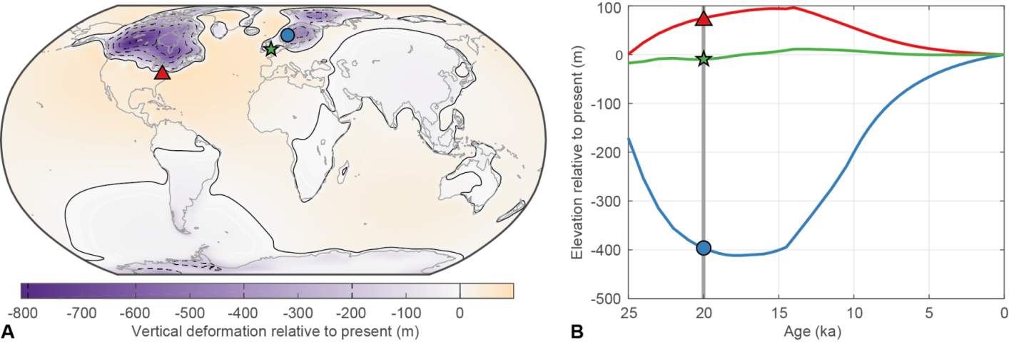
Past land surface elevation change from glacial isostatic adjustment (GIA). A) Global surface elevation relative to today is shown for the peak of the last ice age (20,000 years ago). Zero difference is contoured with a solid black line, while dashed contours are at 200-m intervals. B) The change in elevation is shown at 3 contrasting sites: the red site (triangle) is located beyond an ice sheet margin, the blue site (circle) is located near to the centre of an ice sheet, and the green site (star) is located in an area that has experienced very little surface elevation change due to GIA over this time.
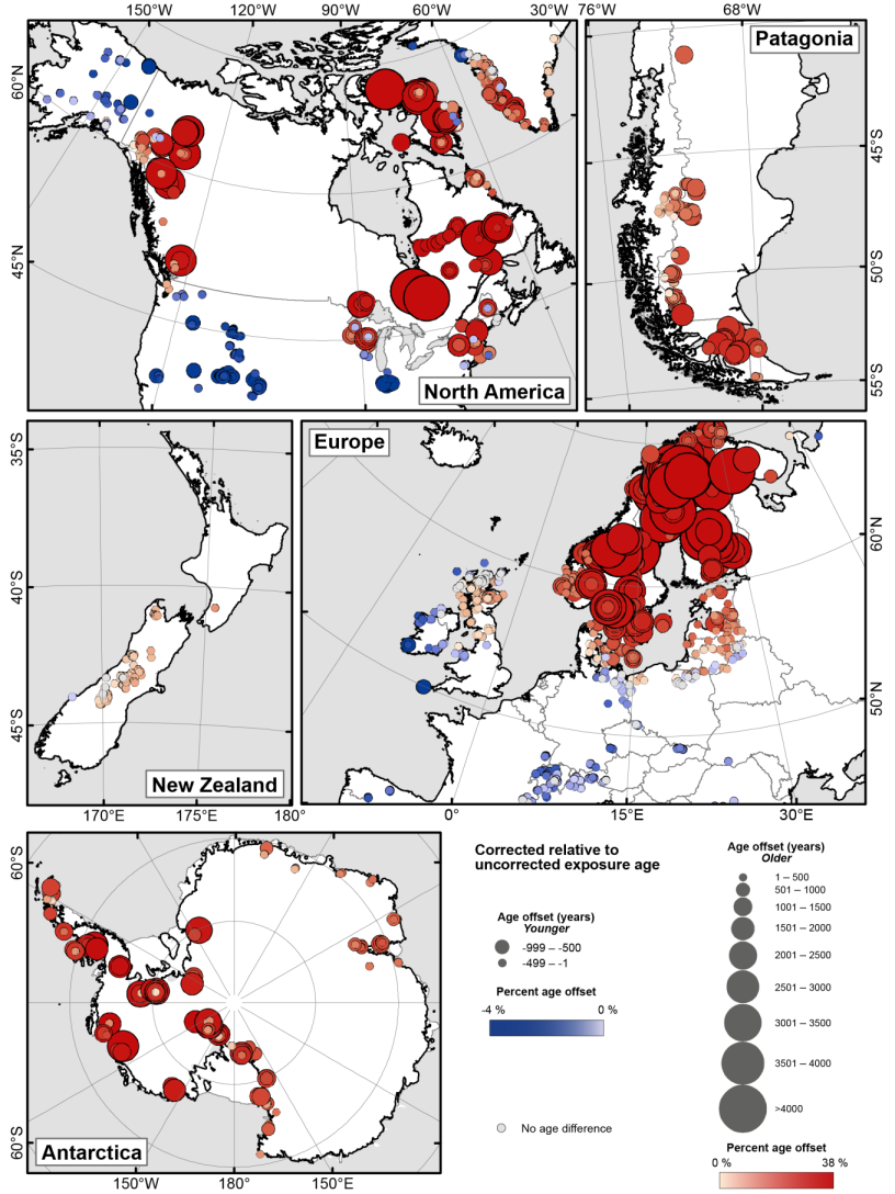
Published surface-exposure ages that were corrected for GIA in Jones et al. (2019). Red symbols highlight ages that become older and blue symbols highlight ages that become younger when accounting for time-dependent GIA effects.
Reference
Jones, R.S., Whitehouse, P.L., Bentley, M.J., Small, D. and Dalton, A.S., 2019. Impact of glacial isostatic adjustment on cosmogenic surface-exposure dating. Quaternary Science Reviews. [DOI: 10.1016/j.quascirev.2019.03.012]
Rates of past ice sheet thinning in Antarctica
11th March 2019
Satellite measurements show us that the Antarctic Ice Sheet is losing ice and, most notably, getting thinner in many places. Predicting how these changes will continue into the future requires advanced computer models that can simulate ice sheet behaviour over 100s to 1000s of years. To improve the accuracy of these models we can test their performance at reproducing past ice sheet changes that are recorded from geological data. Cosmogenic-nuclide surface-exposure dating is a technique that can tell us how long a rock has been exposed at the Earth’s surface. As an ice sheet gets thinner it deposits rocks on mountains emerging from the ice—rocks on the upper slopes will be exposed before rocks on the lower slopes. By dating the time of exposure with surface-exposure dating it is possible to calculate how quickly the ice sheet thinned in the past.
Small et al. compiled existing surface-exposure data from across the Antarctic continent. While some of this data had previously been used to calculate thinning rates, much of it had not. By compiling all the useful data they were able to produce the first continent-wide database of past Antarctic Ice Sheet thinning rates. The rates were produced using the Estimate Linear Rate tool MATLAB code. This compilation shows us that thinning rates in the past—during a time when the ice sheet was shrinking from its maximum extent at the last ice age—are similar to rates observed by satellites today. Additionally, the locations where rapid thinning is recorded in the past appear to broadly match locations where rapid thinning occurs today. These estimates of past ice sheet thinning will next be used to help constrain computer models that are simulating changes in the size and behaviour of the Antarctic Ice Sheet since the last ice age.
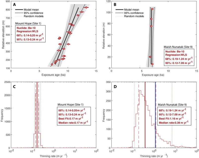
Example thinning rates generated using the Estimate Linear Rate iceTEA tool. Weighted Least Squares linear regression was performed within a Monte Carlo framework, shown here for two vertical sample transects (A and B; Sites 1 and 9). The resulting distribution of modelled thinning rates is then calculated (C and D), at 68% (dashed vertical lines) and 95% (dotted vertical lines) confidence. The mean rate (labelled here as ‘best-fit’) and median rate are shown as blue and red vertical lines, respectively. Note, the mean, median and probability range is much larger at Site 9 (Maish Nunatak).
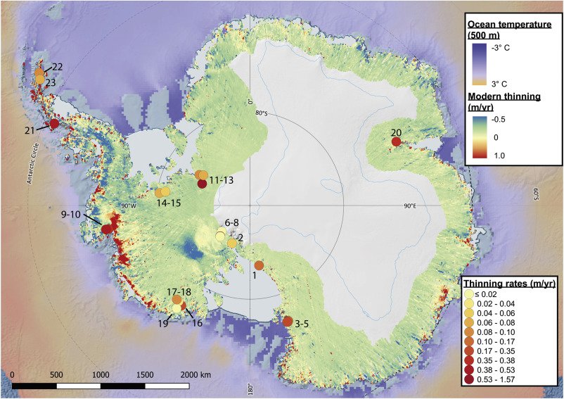
Computed rates of past thinning (circles) are shown against modern thinning rates and present-day ocean temperatures at 500 m depth (produced using Quantarctica GIS package). The rates of past thinning are similar to those observed today, implying that modern thinning has the potential to be sustained for some time into the future.
Reference
Small, D., Bentley, M.J., Jones, R.S., Pittard, M.L. and Whitehouse, P.L., 2019. Antarctic ice sheet palaeo-thinning rates from vertical transects of cosmogenic exposure ages. Quaternary Science Reviews, 206, 65-80. [DOI: 10.1016/j.quascirev.2018.12.024]